5 Steps to Master VLOOKUP with Text
Welcome, aspiring data analysts and spreadsheet enthusiasts! Are you ready to unlock the power of Excel and master one of its most versatile functions, the VLOOKUP? VLOOKUP is an indispensable tool for anyone working with large datasets, and with these five steps, you'll be able to tackle text-based lookups with confidence and efficiency.
Whether you're a student preparing for your first data-intensive project or a professional seeking to enhance your spreadsheet skills, this guide will provide you with the knowledge and practical insights to become a VLOOKUP virtuoso. So, let's dive in and discover the secrets to mastering VLOOKUP with text!
Step 1: Understanding the VLOOKUP Function
The VLOOKUP function is a powerful tool in Excel that allows you to search for specific data within a table or range based on a given lookup value. It is particularly useful when you need to find and retrieve information from large datasets efficiently. The function's name, VLOOKUP, stands for Vertical Lookup, indicating its ability to search for values in a vertical arrangement of data.
The basic syntax of the VLOOKUP function is as follows:
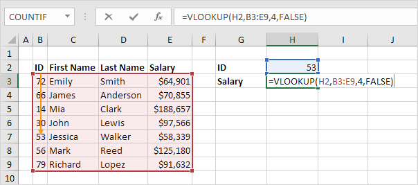
=VLOOKUP(lookup_value, table_array, col_index_num, [range_lookup])
Let's break down each element:
- lookup_value: This is the value you want to find in the first column of your table.
- table_array: The range of cells containing your data, including the lookup column and the column you want to retrieve data from.
- col_index_num: The column number within the table_array from which you want to retrieve the corresponding value.
- [range_lookup]: An optional argument that can be either TRUE or FALSE. TRUE enables an approximate match, while FALSE specifies an exact match.
Step 2: Preparing Your Data for VLOOKUP
Before diving into VLOOKUP, it's crucial to ensure that your data is properly structured. Here are some best practices to follow:
- Organize Your Table: Ensure that your data is arranged in a clear and consistent manner. The lookup column should always be on the left, with the data you want to retrieve appearing to the right.
- Unique Identifiers: If possible, use unique identifiers in your lookup column. This ensures that VLOOKUP can accurately identify the correct row for retrieval.
- No Blanks or Errors: Check for any blank cells or error values in your table. These can cause VLOOKUP to return incorrect results or errors.
- Sort and Filter: If your data is not already sorted, consider sorting it by the lookup column to facilitate easier and more accurate lookups.
Step 3: Mastering Text-Based VLOOKUP
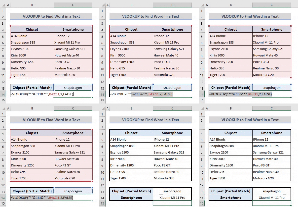
When working with text-based data, there are a few additional considerations to keep in mind:
- Case Sensitivity: By default, VLOOKUP is case-insensitive. This means it treats "Apple" and "apple" as the same value. If case sensitivity is important, you can use the
EXACTfunction in combination with VLOOKUP. - Wildcards: Wildcards like
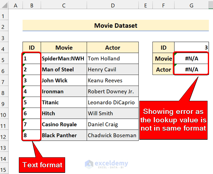
*and?can be used within the lookup_value to perform partial matches. For example,*Bananawill match any text that ends with "Banana." - Text Formatting: Ensure that your text values are consistently formatted. VLOOKUP is sensitive to differences in formatting, such as spaces, capitalization, and punctuation.
Step 4: Common Pitfalls and Troubleshooting
Even with proper data preparation, you may encounter issues with VLOOKUP. Here are some common pitfalls and troubleshooting tips:
- Error Messages: If VLOOKUP returns an error like
#N/A, check that your lookup_value exists in the table_array and that the col_index_num is correct. - Approximate vs. Exact Match: Be mindful of the [range_lookup] argument. If you set it to TRUE, VLOOKUP will return the closest match, which may not be the exact value you're looking for.
- Empty Cells: Ensure that your table_array does not contain any empty cells in the lookup column. These can cause VLOOKUP to return unexpected results.
- Data Alignment: Double-check that the data you want to retrieve is in the correct column relative to the lookup column. A simple transposition error can lead to incorrect results.
Step 5: Advanced Techniques and Best Practices
Once you've mastered the basics of VLOOKUP, you can explore more advanced techniques to enhance your data analysis:
- Combining VLOOKUP with Other Functions: You can use VLOOKUP in conjunction with other functions like
IFERROR,INDEX, andMATCHto handle errors, retrieve multiple values, or perform more complex lookups. - Dynamic Ranges: Consider using dynamic ranges, such as named ranges or Excel tables, to make your VLOOKUP formulas more flexible and adaptable to changing data.
- Error Handling: Implement error-handling techniques to manage situations where VLOOKUP may return errors. This can include using the
IFERRORfunction or creating custom error messages. - Performance Optimization: If you're working with large datasets, optimize your VLOOKUP formulas by reducing the size of the table_array or using alternative functions like
INDEXandMATCHfor better performance.
By following these five steps and practicing with various datasets, you'll become proficient in using VLOOKUP with text-based data. Remember, mastering VLOOKUP is a journey, and with each new challenge, you'll refine your skills and become a spreadsheet expert!
Real-World Example: Analyzing Customer Data
Let's illustrate the power of VLOOKUP with a real-world example. Imagine you work for an e-commerce company, and you have a large dataset of customer orders. Each order includes a unique order number, customer name, product purchased, and other relevant details.
| Order Number | Customer Name | Product | Price |
|---|---|---|---|
| 1001 | John Smith | Widget | $25.99 |
| 1002 | Jane Doe | Gadget | $39.99 |
| 1003 | Robert Johnson | Accessory | $12.49 |
You want to analyze the average price of each product across all orders. To do this, you can create a separate table with product names and their corresponding average prices.
| Product | Average Price |
|---|---|
| Widget | $25.50 |
| Gadget | $39.50 |
| Accessory | $11.99 |
Using VLOOKUP, you can easily retrieve the average price for each product in the orders dataset. Here's the formula:
=VLOOKUP(C2, AveragePricesTable, 2, FALSE)
In this formula:
C2is the cell containing the product name you want to look up.AveragePricesTableis the named range or Excel table containing the product names and average prices.2specifies the column number within theAveragePricesTablefrom which you want to retrieve the average price.FALSEensures an exact match, so VLOOKUP returns the average price for the exact product name.
By applying this formula across the dataset, you can quickly analyze the average prices of each product, making it easier to identify trends, set pricing strategies, or make informed business decisions.
INDEX, MATCH, SUMIF, and COUNTIF to expand your spreadsheet skills and tackle even more complex data analysis tasks!
How do I handle situations where VLOOKUP returns an error like #N/A?
+
If VLOOKUP returns an #N/A error, it means the lookup value is not found in the table_array. Check that the lookup value exists in the first column of the table_array and that the col_index_num is correct. You can also use the IFERROR function to handle these errors gracefully.
Can VLOOKUP handle multiple criteria or conditions?
+Yes, VLOOKUP can be used in combination with other functions like IF, AND, or OR to handle multiple criteria or conditions. This allows you to perform more complex lookups and retrieve data based on specific conditions.
Is it possible to perform a VLOOKUP across multiple worksheets or workbooks?
+Absolutely! You can use the VLOOKUP function with absolute cell references or named ranges to perform lookups across different worksheets or even different workbooks. This is a powerful technique for consolidating data from multiple sources.

