5 Excel Left Join Tips
Excel, the ubiquitous spreadsheet software, is a powerful tool for data analysis and manipulation. Among its many features, the ability to perform joins, particularly the left join, is invaluable for merging datasets and creating comprehensive analyses. In this article, we will explore five expert tips to master the art of left joins in Excel, providing you with the knowledge to tackle complex data tasks with ease.
Understanding the Left Join
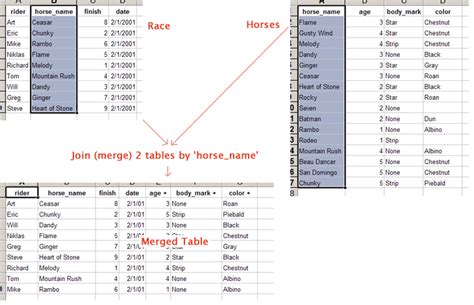
A left join, also known as a left outer join, is a fundamental operation in relational databases and spreadsheet applications like Excel. It combines rows from two datasets based on a common field or key, ensuring that all records from the left table are included in the result, even if there are no corresponding matches in the right table. This makes it an essential tool for data analysts, researchers, and anyone working with datasets that need to be merged or reconciled.
In Excel, the left join is particularly useful when you have two datasets that you want to combine, especially when one dataset is a master list or a primary source of information, and the other provides additional details or updates. By using a left join, you can retain all the records from the primary dataset and fill in any missing data from the secondary dataset, creating a comprehensive, unified view of your information.
Tip 1: Prepare Your Data

Before performing a left join, it’s crucial to ensure your data is properly prepared. This means that the columns you intend to join should have identical data types and formats. For instance, if you’re joining on a date field, ensure that both columns are formatted consistently as dates, not as text or some other format.
Additionally, ensure that your data is free of any errors or inconsistencies. Check for duplicate records, missing values, or incorrect data entries. Excel's data cleaning tools, such as the Remove Duplicates feature and the Find and Replace function, can be invaluable in preparing your data for a successful left join.
Example Data Preparation
Let’s say you have a dataset of customer orders, with a column named “CustomerID”, and you want to merge it with a customer details dataset that also has a “CustomerID” column. Before performing the left join, you should:
- Ensure that both “CustomerID” columns are formatted as text to avoid any automatic number formatting by Excel.
- Check for any duplicate “CustomerID” values and remove them to avoid potential errors in the join.
- Scan for any missing values in the “CustomerID” column and either fill in the missing information or handle these cases separately in your join.
Tip 2: Use the VLOOKUP Function for Simple Joins
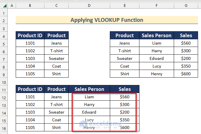
For straightforward left joins, Excel’s VLOOKUP (Vertical Lookup) function is a quick and efficient solution. This function allows you to search for a value in the leftmost column of a range of cells and return a value from the same row in a column you specify.
When using VLOOKUP for a left join, ensure that your data is sorted in ascending order based on the key field you're joining on. This ensures that Excel can efficiently find the corresponding values in the right table.
VLOOKUP Syntax
The syntax for the VLOOKUP function is as follows:
=VLOOKUP(lookup_value, table_array, col_index_num, [range_lookup])
- lookup_value: This is the value you want to find in the leftmost column of the table.
- table_array: This is the range of cells that contains the data you want to search.
- col_index_num: This is the column number in the table_array from which the matching value must be returned.
- range_lookup: This is an optional value that specifies whether you want an exact or approximate match. Set it to FALSE for an exact match, which is typically what you want for a left join.
Example VLOOKUP Usage
Suppose you have two datasets: Orders and Customers, and you want to retrieve the customer name from the Customers dataset based on the CustomerID in the Orders dataset. You can use the following VLOOKUP formula:
=VLOOKUP(B2, Customers, 2, FALSE)
Where B2 contains the CustomerID from the Orders dataset, and the Customers dataset is arranged as CustomerID in the leftmost column followed by the Customer Name column.
Tip 3: Power Query for Advanced Joins
Excel’s Power Query tool, introduced in Excel 2010, is a powerful feature for data transformation and manipulation. It provides a user-friendly interface to perform various data operations, including joins, and can handle large datasets with ease.
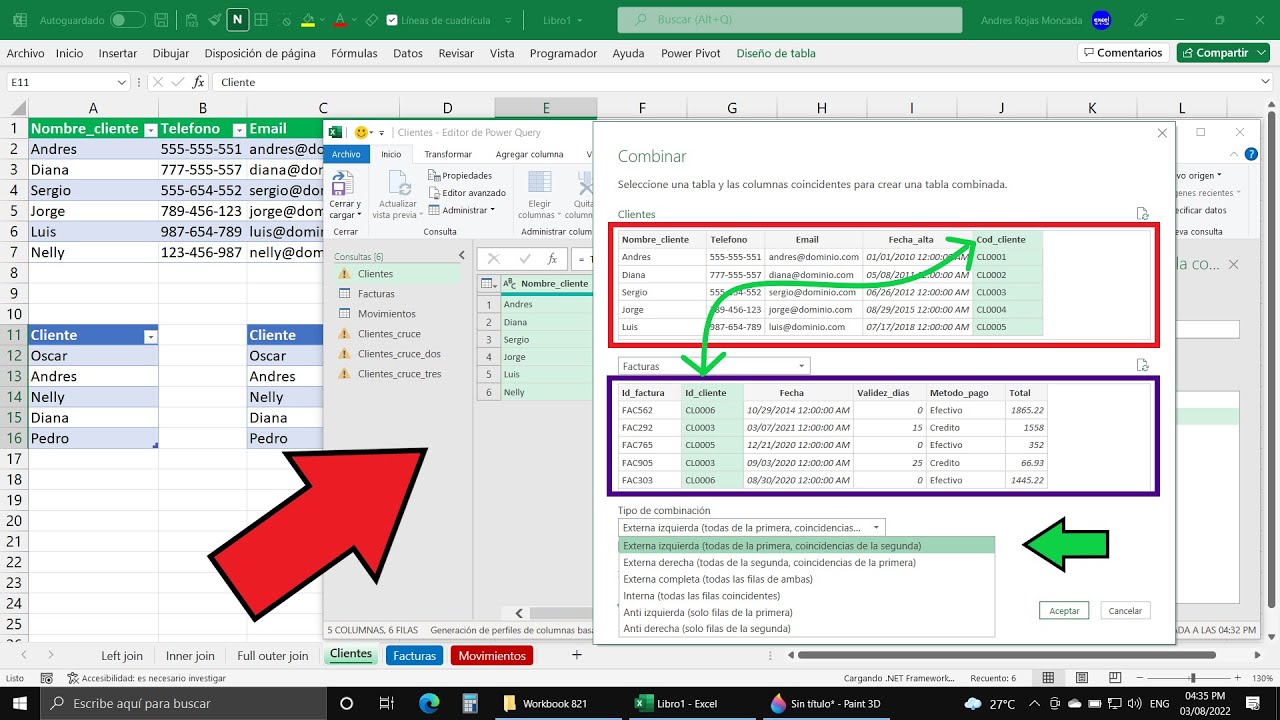
To perform a left join using Power Query, you first need to load your data into the Power Query Editor. Then, you can follow these steps:
- In the Power Query Editor, select the table you want to perform the join on (the left table), and click on Home > Join.
- Select Left Outer as the join kind.
- Choose the table you want to join with (the right table) and select the columns to be joined.
- Define the matching criteria. This is the column or field that will be used to match records between the two tables.
- Click OK to perform the join and load the results back into Excel.
Advantages of Power Query
- Flexibility: Power Query allows you to perform more complex joins, including joins on multiple fields or columns, and can handle datasets with different data types.
- Data Refresh: Once you've established a connection between your datasets using Power Query, you can easily refresh the data to get the latest information without performing the join again.
- Error Handling: Power Query provides robust error handling capabilities, allowing you to manage potential issues that might arise during the join process.
Tip 4: Combine VLOOKUP with IFERROR for Error Handling
While the VLOOKUP function is powerful, it can return an error if it doesn't find a match in the right table. To handle this scenario gracefully, you can combine VLOOKUP with the IFERROR function. The IFERROR function allows you to specify what should happen if an error occurs in another formula.
IFERROR Syntax
The syntax for the IFERROR function is as follows:
=IFERROR(value, value_if_error)
- value: This is the formula or value you want to check for errors.
- value_if_error: This is the value or formula that should be returned if an error is found in the value argument.
Example IFERROR Usage
Combining VLOOKUP with IFERROR, you can return a custom message or value if a match isn’t found. For instance:
=IFERROR(VLOOKUP(B2, Customers, 2, FALSE), “Customer not found”)
In this example, if the VLOOKUP function doesn’t find a match, it will return “Customer not found” instead of an error.
Tip 5: Use Advanced Filter for Large Datasets
For larger datasets, using Excel’s Advanced Filter feature can be more efficient than VLOOKUP or Power Query. The Advanced Filter allows you to copy and paste unique records that meet specific criteria from one range to another.
To perform a left join using the Advanced Filter, you first need to ensure that your left and right tables have a common key field. Then, you can follow these steps:
- Select the range of cells that contains your left table, including the headers.
- Go to Data > Advanced.
- In the Advanced Filter dialog box, select Copy to another location and specify the range for the output.
- In the List range field, specify the range of your left table.
- In the Criteria range field, specify the range of your right table. Ensure that the column you’re joining on in the right table is the first column in the criteria range.
- Check the Unique records only box to ensure that only unique matches are copied.
- Click OK to perform the filter and create your joined dataset.
Advanced Filter Advantages
- Efficiency: The Advanced Filter can handle large datasets more efficiently than some other methods, especially if your join key is the first column in your right table.
- Speed: For simple left joins, the Advanced Filter can provide faster results compared to other methods.
- Simplicity: While it might not offer the same flexibility as Power Query, the Advanced Filter is a straightforward and quick way to perform a left join, especially for those familiar with Excel’s traditional functions.
| Join Method | Advantages | Disadvantages |
|---|---|---|
| VLOOKUP | Simple and straightforward for basic joins | Can't handle complex joins, prone to errors without proper error handling |
| Power Query | Flexible and powerful, can handle complex joins and large datasets | Steep learning curve for beginners, requires data to be loaded into the Power Query Editor |
| Advanced Filter | Efficient for large datasets, fast and simple to use | Limited flexibility compared to Power Query, not suitable for complex joins |
FAQs
Can I perform a left join if my data is not sorted?
+
Yes, but it’s generally recommended to sort your data based on the join key before performing a left join. This ensures that Excel can efficiently find the corresponding values in the right table.
What happens if I have duplicate records in my left table or right table?
+
In a left join, duplicate records in the left table will be treated as separate records, each joined with the corresponding record in the right table. If there’s no corresponding record in the right table, the missing data will be filled with N/A or another specified value.
Can I perform a left join if my data is in different Excel files or workbooks?
+
Yes, you can. You’ll need to use the VLOOKUP function or Power Query to reference the data from the external file or workbook. Make sure to establish a connection to the external data source if you’re using Power Query.


