Excel Magic: 5 Conditional Formatting Tips
Conditional formatting in Excel is a powerful tool that allows users to dynamically format cells based on specific conditions or criteria. This feature adds a layer of visual analysis to your data, helping you identify patterns, trends, and outliers with ease. In this article, we will explore five expert tips for mastering conditional formatting, offering insights and techniques to enhance your data presentation and analysis skills.
1. Utilizing Data Bars and Color Scales for Quick Visual Insights
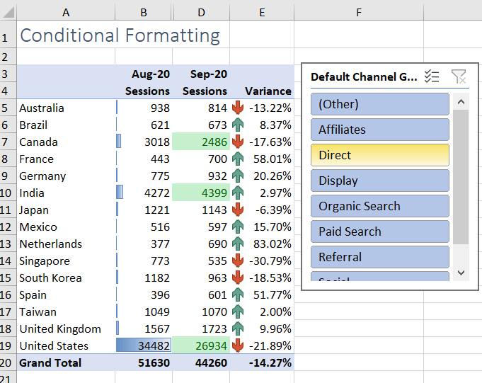
Data bars and color scales are two of the most visually appealing and informative conditional formatting options in Excel. Data bars provide a quick glance at the relative magnitude of values within a dataset. When applied to a range of cells, each cell displays a bar that represents the value in relation to the other cells. This format is especially useful for comparing values at a glance.
Color scales, on the other hand, use a gradient of colors to represent the values in a dataset. Cells with higher values are assigned a darker shade, while lower values receive a lighter shade. This format is ideal for identifying clusters of similar values or outliers in your data.
To apply these formats, simply select the data range, navigate to the “Home” tab, and choose either “Data Bars” or “Color Scales” from the “Conditional Formatting” dropdown menu. Excel offers a range of default options, but you can also customize the colors and scales to suit your preferences or the specific nature of your data.
Example: Visualizing Sales Performance
Imagine you have a sales dataset with columns for Product, Quantity Sold, and Revenue. By applying data bars to the Quantity Sold column, you can quickly identify the top-selling products without even reading the numbers. Similarly, using a color scale on the Revenue column can highlight high-revenue products in darker shades, making it easy to spot profitable items.
| Product | Quantity Sold | Revenue |
|---|---|---|
| Widget A | 150 | $2,500 |
| Widget B | 200 | $3,200 |
| Widget C | 50 | $1,200 |
2. Creating Icon Sets for Enhanced Data Visualization

Icon sets provide a unique and intuitive way to visualize data. With icon sets, you can represent values or conditions using a set of icons, such as arrows, ratings, or directional symbols. This format is particularly effective for communicating data trends or performance indicators to a broad audience, including those who may not be familiar with Excel.
To apply icon sets, select the desired data range, navigate to the “Home” tab, and choose “Icon Sets” from the “Conditional Formatting” dropdown menu. Excel offers a variety of icon set options, including arrows, ratings, and directional symbols. You can also customize the icons and their associated values to align with your data and analysis goals.
Example: Visualizing Customer Satisfaction
Consider a dataset containing customer feedback and satisfaction scores. By applying an icon set that uses smiley faces to represent satisfaction levels, you can quickly convey the overall sentiment of your customers. For instance, a five-star icon set can visually represent high satisfaction, while a one-star icon set indicates low satisfaction.
| Customer | Satisfaction Score | Icon Set |
|---|---|---|
| Alice | 4.8 | 🌟🌟🌟🌟🌟 |
| Bob | 3.2 | 🌟🌟🌟 |
| Carol | 5.0 | 🌟🌟🌟🌟🌟 |
3. Mastering the Art of Formulas in Conditional Formatting
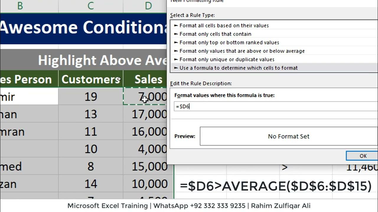
While Excel offers a range of pre-defined conditional formatting options, the real power lies in your ability to craft custom formulas. With custom formulas, you can create highly specific and dynamic formatting rules that adapt to your data’s unique characteristics.
To apply custom formulas, select the data range, navigate to the “Home” tab, and choose “New Rule” from the “Conditional Formatting” dropdown menu. From here, you can select “Use a formula to determine which cells to format” and enter your custom formula. This formula can refer to other cells, use Excel functions, and even leverage complex logic to define the formatting conditions.
Example: Flagging Duplicate Values
Imagine you have a dataset with a column containing customer IDs. To flag potential duplicate entries, you can use a custom formula. For instance, the formula =COUNTIF(B2:B100,B2)>1 will identify duplicates in the Customer ID column. Applying conditional formatting with this formula will highlight cells containing duplicate IDs, helping you quickly identify and address any data errors.
| Customer ID | Name | Address |
|---|---|---|
| 12345 | Alice | 123 Main St |
| 67890 | Bob | 456 Pine Ave |
| 12345 | Carol | 789 Oak Rd |
4. Applying Conditional Formatting to Multiple Sheets for Consistent Visualization
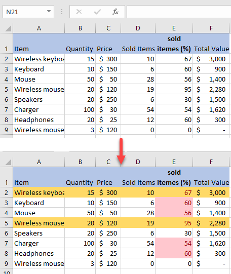
When working with multiple sheets or workbooks, maintaining consistent data visualization can be a challenge. Conditional formatting can help by allowing you to apply the same formatting rules across different sheets or workbooks.
To apply conditional formatting to multiple sheets, first apply the desired formatting to the data on your active sheet. Then, select the “Format” tab in the “Conditional Formatting” dropdown menu. From here, you can choose “Apply to Other Sheets” and select the desired sheets or workbooks to apply the same formatting.
Alternatively, you can create a Formatting Rule in the “New Formatting Rule” dialog box and then apply this rule to multiple sheets. This approach ensures that any changes made to the rule will automatically update across all selected sheets.
Example: Standardizing Financial Reports
Suppose you have monthly financial reports for your company, with each month on a separate sheet. By applying the same conditional formatting rules to highlight key financial metrics (e.g., profit margins, revenue growth), you can ensure a consistent and easily understandable visualization across all sheets. This standardization makes it easier to compare and analyze financial performance over time.
5. Using Conditional Formatting with Data Validation for Enhanced Data Integrity

Data validation and conditional formatting are powerful tools that can be used in conjunction to enhance data integrity and user experience in Excel. Data validation allows you to specify rules for what data is acceptable in a cell or range of cells, while conditional formatting can provide visual cues to users about the validity of their data entries.
To combine data validation with conditional formatting, first set up the data validation rules for the desired cells or range. Then, create a conditional formatting rule that checks for errors or specific conditions based on the data validation rules. This way, you can highlight invalid data entries or provide visual feedback to users, helping them make accurate data entries.
Example: Ensuring Correct Date Entries
Consider a scenario where you’re collecting data for a project with a specific deadline. By setting up data validation to allow only dates within a certain range (e.g., the project duration), you can ensure that data entries are valid. Additionally, you can use conditional formatting to highlight cells with invalid dates in red, providing a visual cue to users that their entry needs to be corrected.
| Task | Deadline |
|---|---|
| Research | 2023-09-15 |
| Design | 2023-09-20 |
| Implementation | 2023-09-25 |
Conclusion
Conditional formatting is a versatile and powerful tool in Excel that can significantly enhance your data analysis and visualization capabilities. By mastering these five tips, you can leverage the full potential of conditional formatting to create insightful and visually appealing data presentations. Remember to experiment, customize, and adapt these techniques to suit your specific data needs and analysis goals.
How do I remove conditional formatting in Excel?
+
To remove conditional formatting, select the cells or range with the formatting, navigate to the “Home” tab, and choose “Clear” from the “Conditional Formatting” dropdown menu. Then, select “Clear Rules” and choose the appropriate option based on whether you want to clear rules from only the selected cells or from the entire sheet.
Can I copy conditional formatting rules when copying and pasting data?
+
Yes, you can copy conditional formatting rules along with your data. When copying and pasting data, ensure that the “Paste Special” option is selected, and then choose “Paste Special” > “All” > “All Using Source Theme”. This will paste both the data and the conditional formatting rules from the source cells to the destination cells.
How do I edit existing conditional formatting rules in Excel?
+
To edit existing conditional formatting rules, select the cells or range with the formatting, navigate to the “Home” tab, and choose “Manage Rules” from the “Conditional Formatting” dropdown menu. From here, you can edit, delete, or create new rules for the selected cells.
