Master Excel: Color Rows with Cell-Based Rules

Excel, a powerful tool in the Microsoft Office suite, is renowned for its ability to organize, analyze, and visualize data. One of its most useful features is the ability to apply conditional formatting, allowing users to highlight specific data points or patterns within a spreadsheet. This article will delve into the process of mastering Excel's conditional formatting by focusing on how to color rows based on cell-based rules, a technique that can significantly enhance data readability and facilitate complex data analysis.
Understanding Conditional Formatting in Excel

Conditional formatting is a versatile Excel feature that allows users to apply specific formatting to cells based on their content or values. This formatting can include font styles, borders, and, most notably for this discussion, cell or row colors. The power of conditional formatting lies in its ability to automatically adjust the visual presentation of data based on predefined rules, making it an invaluable tool for data analysts, accountants, researchers, and anyone working with large datasets.
The Benefits of Cell-Based Row Coloring
Coloring rows based on cell values is an effective strategy for data visualization, especially when dealing with large tables. This technique draws attention to specific data points, making it easier to identify trends, anomalies, or key insights. For instance, a financial analyst might use cell-based row coloring to highlight rows where a particular metric exceeds a certain threshold, making it simpler to spot potential areas of concern or opportunity.
Step-by-Step Guide: Coloring Rows with Cell-Based Rules

Mastering the art of conditional formatting can significantly enhance your Excel skills and data presentation. Here’s a detailed guide on how to color rows based on cell values.
Step 1: Select the Data Range
Begin by selecting the data range you want to format. This could be a single column, multiple columns, or even an entire table. Ensure that your data is organized and consistent, as conditional formatting relies on clear data structures.
Step 2: Access the Conditional Formatting Menu
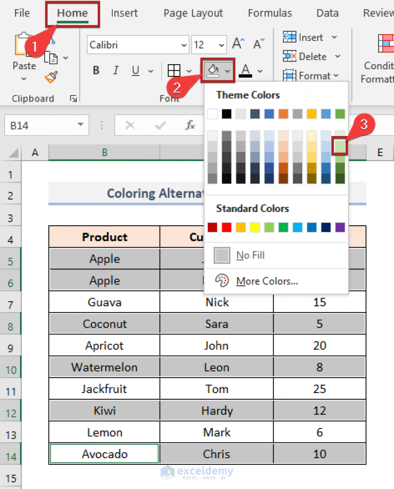
Navigate to the Home tab in the Excel ribbon. Within the Styles group, you’ll find the Conditional Formatting dropdown. Click on this to reveal a menu of pre-set rules and custom formatting options.
Step 3: Choose a Rule Type
Excel offers a variety of rule types to suit different data scenarios. Some common rule types include:
- Highlight Cells Rules: Allows you to highlight cells based on their value, text, or date.
- Top/Bottom Rules: Formats the top or bottom percentage of values in a range.
- Data Bars: Displays data bars within cells to visually compare values.
- Color Scales: Applies a color scale to cells based on their values.
- Icon Sets: Uses icons to represent the values in a range.
Step 4: Define Your Rule
Once you’ve chosen a rule type, you’ll need to define the parameters of your rule. For example, if you’re using a Highlight Cells Rule, you can set a condition such as “greater than” a specific value, and then select a fill color to apply to cells that meet this condition.
Step 5: Apply the Formatting
With your rule defined, simply click OK to apply the formatting to your selected data range. Excel will automatically adjust the row colors based on the values in the cells.
Step 6: Fine-Tune and Customize
Excel’s conditional formatting offers a high degree of customization. You can adjust the rule settings, create multiple rules for a single range, and even manage the priority of rules to ensure they apply correctly. Additionally, you can use the Manage Rules feature to edit, delete, or move rules to different ranges.
Advanced Techniques: Dynamic Row Coloring
Mastering conditional formatting opens up a world of advanced techniques for data visualization and analysis. One such technique is dynamic row coloring, where the color of a row changes based on the value of a specific cell within that row.
Using Formulas in Conditional Formatting
Excel’s conditional formatting can be enhanced with formulas, allowing for more complex and dynamic rule definitions. For example, you might use a formula to compare values in different cells, or to perform calculations before applying a formatting rule.
| Formula | Description |
|---|---|
| =AVERAGE(B2:B10) | Calculates the average of values in cells B2 to B10. |
| =SUM(IF(B2:B10>"Target",1,0)) | Counts the number of cells in B2 to B10 that are greater than "Target". |
| =COUNTIF(B2:B10,">100") | Counts the number of cells in B2 to B10 that are greater than 100. |

Dynamic Row Coloring Example
Consider a scenario where you have a sales report with columns for Product, Quantity Sold, and Price per Unit. You want to color-code the rows based on the Quantity Sold, but only if the Price per Unit is above a certain threshold. Here’s how you could achieve this:
- Select the range of cells you want to format (in this case, the entire table).
- Go to the Home tab and choose Conditional Formatting from the Styles group.
- Select New Rule and choose Use a formula to determine which cells to format.
- In the formula bar, enter
=B2>10, whereB2represents the Quantity Sold for the first row. - Click Format and choose a fill color for rows that meet this condition.
- Click OK to apply the rule.
- Now, if the Quantity Sold in any row is greater than 10, and the Price per Unit is above the threshold you've set, that row will be color-coded.
Best Practices and Considerations
While conditional formatting is a powerful tool, it’s important to use it judiciously to maintain data clarity and readability. Here are some best practices to keep in mind:
- Consistency: Ensure that your formatting rules are consistent throughout your spreadsheet to avoid confusion.
- Clarity: Choose colors that are easy to distinguish and don't overwhelm the data.
- Manage Complexity: Too many rules can make your spreadsheet difficult to manage. Use the Manage Rules feature to keep track of your rules and ensure they're applied correctly.
- Print Considerations: When preparing a spreadsheet for printing, be mindful of how conditional formatting will appear on paper. You may need to adjust your rules or add additional formatting for printed documents.
Conclusion: Mastering Data Visualization with Excel

Conditional formatting, particularly the technique of coloring rows based on cell values, is a powerful tool for data visualization and analysis in Excel. By mastering this feature, you can transform complex datasets into visually appealing and informative spreadsheets, making it easier to identify trends, patterns, and key insights. With the right techniques and best practices, Excel’s conditional formatting can significantly enhance your data analysis capabilities.
How can I remove conditional formatting from a range of cells in Excel?
+
To remove conditional formatting from a range of cells, select the cells and navigate to the Home tab. In the Styles group, click on Conditional Formatting and select Clear Rules. From the dropdown menu, choose whether you want to clear the rules from the selected cells or the entire sheet.
Can I apply multiple conditional formatting rules to a single cell or range of cells in Excel?
+
Yes, you can apply multiple conditional formatting rules to a single cell or range of cells. Excel allows you to create and manage a list of rules for a selected range. The order of the rules matters, as Excel applies the rules in the order they’re listed. If a cell meets the conditions of multiple rules, only the formatting of the first applicable rule will be applied.
Is there a way to copy conditional formatting rules from one cell or range to another in Excel?
+
Absolutely. Excel provides a convenient way to copy conditional formatting rules. Simply select the cell or range with the formatting you want to copy, then use the Format Painter tool (it looks like a paintbrush) from the Home tab. Click on the cell or range where you want to apply the formatting, and it will be copied.


